Estimating the Diversity Score of a Portfolio across Multiple Correlated Sectors: Generalized Herfindahl-Hirschman Index

Diversification is an effective risk mitigation strategy for portfolio risk management. It helps to mitigate risk arising from various factors, including extreme events, except factors which are systemic in nature. Often diversification across counterparties, sectors or geographies is the only risk mitigation tool available to a credit portfolio manager. It is important to measure and monitor the degree of diversification periodically to ensure that concentration risk remains low. However, quantifying the diversification may not be straightforward. Herfindahl-Hirschman Index (HHI) is one such measure but has limitations as it does not take into account correlation among underlying assets. In this post, we discuss a more general and effective measure of diversity score, Generalized-HHI (GHHI), to quantify diversification of a portfolio across multiple correlated sectors and sub-sectors.

In this post we first give a brief overview of how diversification helps to mitigate risk. We also discuss briefly the effect of correlation on portfolio risk. Next, we give a quick introduction to the classical HHI measure. In the last sections we present the GHHI formulation and illustrate its usage to identify a best diversified portfolio. In this blog post, we do not discuss in detail the derivation of GHHI and request interested readers to refer to the Working Paper for a detailed discussion.

How Diversification Helps

We discuss the benefit of diversification using a hypothetical credit portfolio of INR 1000 which can be lent to a single or multiple borrowers. Let us assume that all borrowers have an annual default probability (PD) of 5%. The portfolio manager has three options to lend the entire amount to:

(a) Scenario 1- A single borrower – No diversification
(b) Scenario 2- Equally to ten borrowers with no default correlation among them
(c) Scenario 3- Equally to ten borrowers with a pairwise default correlation of 0.33 among them

Assume no recovery.

Assuming 5% PD for each borrower, the expected loss of the portfolio in all scenarios is same and is equal to INR 50. However, the unexpected risk, measured as the standard deviation of loss here, for the three portfolios will be different.

The loss distributions of Scenario 1 and Scenario 2 are shown in the Figure 1. Scenario 1 has higher standard deviation because it has probabilities bunched only towards the ‘INR 0 loss’ and ‘INR 1000 Loss’ events which is intuitive for a one borrower portfolio- either all good or all bad, whereas a diversified portfolio, under scenario 2, has a better distribution with a very thin tail. For example, under Scenario 2 the probability of INR 1000 loss is nearly 1 in 10,000,000,000,000 as opposed to 1 in 20 in Scenario 1. Remember that Scenario 2 assumes no correlation among borrowers.

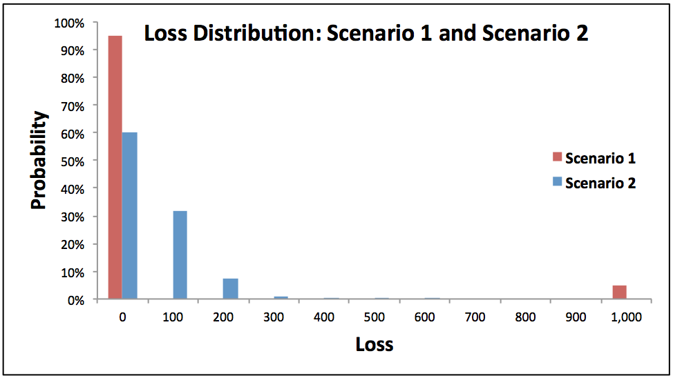
Figure 1: Loss Distribution: Scenario 1 and Scenario 2

Let’s see how correlation impacts the loss distribution. The loss distribution of Scenario 2 and Scenario 3 are compared in Figure 2. It can be seen that the latter’s loss distribution has fatter tails. The probability under Scenario 3 of INR 1000 loss is nearly 1 in 240, much higher than that under Scenario 2 but lower than that under no diversification Scenario 1. This tells us that greater than zero default correlation among borrowers increase risk in the portfolio and should be taken into account while quantifying the degree of diversification.

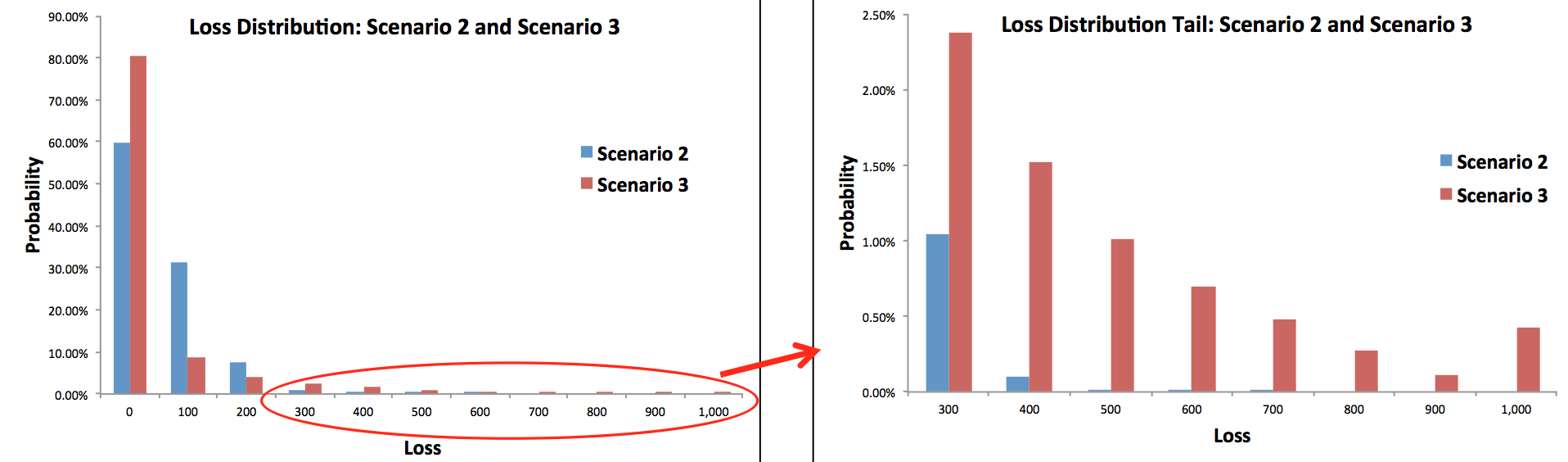
Figure 2: Loss Distribution: Scenario 2 and Scenario 3

Herfindahl-Hirschman Index (HHI)

One commonly used method of measuring the degree of diversification is HHI. HHI is defined as sum of the squares of the portfolio proportions. Consider a loan portfolio P with exposure across 3 counterparties, $latex C_i&s=1$, with corresponding proportions, $latex c_i&s=1$, where $latex i$ = 1 to 3. Then the degree of diversification for P across counterparties can be measured using HHI, where HHI is:

However, the HHI assumes the sectors are independent and does not take into account the correlation among them. We propose a more general metric, the Generalized Herfindahl-Hirschman Index (GHHI), which incorporates correlation among underlying assets.

Generalized Herfindahl-Hirschman Index (GHHI)

The GHHI formulation for a portfolio P with across n assets having pair wise correlation of $latex \rho_{ij}&s=1$ can be written as:

The derivation of the above formulation is not discussed here for the sake of brevity. We request the reader to refer to the Working Paper for a detailed account.

GHHI Vs HHI – Illustration

As an illustration the HHI and GHHI are estimated for four hypothetical credit portfolios, A, B, C, and D, with exposure in 12 counterparties across three sectors S1, S2 and S3. The counterparties are pairwise correlated within a sector with correlations of 0.05, 0.25 and 0.5 respectively. It is assumed that sectors are pairwise uncorrelated. Column 4 to 6 of Table 1 shows the exposure of the four portfolios in different counterparties.

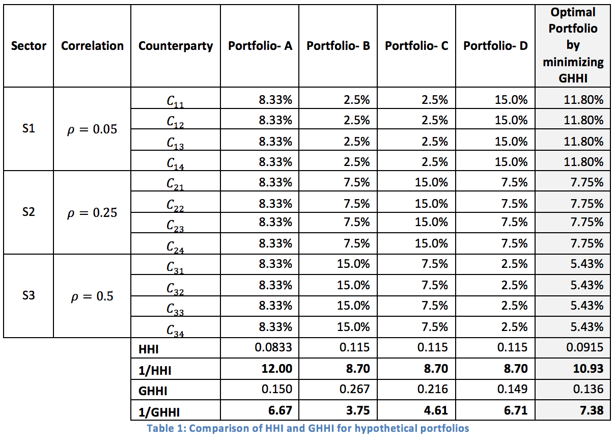
Portfolio A is a seemingly perfectly diversified portfolio with equal exposure to all the available counterparties. In fact, a comparison based on the classic HHI yields a similar conclusion. However, it is shown using GHHI that a more diversified portfolio can be created taking into account the correlation among the counterparties in a sector. The last two rows of Table 1 show the calculated value of diversity scores of each portfolio as well as the effective number of counterparties in each portfolio. Based on HHI, the degree of diversification of the portfolios follows the order: A > B = C = D. Whereas GHHI takes into account the correlation and provides a more accurate order: D > A > C > B, i.e. a portfolio with exposures skewed towards a highly correlated sector, such as S3, will have lower risk mitigation.

Finally, we minimize the GHHI to identify the optimum proportions across assets for the best diversification. The optimal proportions across different sector are indicated in the last column of Table 1.

For a more detailed perspective on this subject please do refer our working paper which you can access here.