
Loan repayment behaviour differs across asset classes based on borrower profile, purpose of loan, geography and nature of security, if any. Certain asset classes show regular and timely repayments with close to 99% collection efficiency but low recovery once a loan reaches a certain delinquency level, say DPD30 (Days past due). On the other hand, there are asset classes with low periodic collection efficiency ranging from 90% to 95%, but ultimate loss on the portfolio may be significantly smaller as compared to the peak delinquency levels showing higher recoveries on delinquent loans. Such differences in repayment behaviour may be driven by cash flow and income volatility of the underlying borrowers as well as delinquency management practices of the lenders among other things. As a result, periodic cash flow shortfalls (or excess) may vary significantly from ultimate loss on the portfolio.
In order to model cash flows accurately, a methodology should be able to model the transitions of loans across different delinquency levels during the tenure. The TM-LGD is one such methodology which does this by first converting the periodic credit behaviour of loans into a ‘transition matrix’ (or TM) and then estimating the periodic cash flows and loss given default (LGD) using Monte-Carlo simulations. Based on the repayment behaviour, a loan may move across different states (delinquent, current, prepaid or pre-closed). Capturing this movement is helpful in estimating the periodic cash flows and ultimate loss on a portfolio. TM captures these transitions across different states using the historical repayment behaviour of the borrowers. Possible transitions for a loan are shown in Figure 1 below. Figure 2 shows an illustrative transition matrix for transitions over a single repayment period.
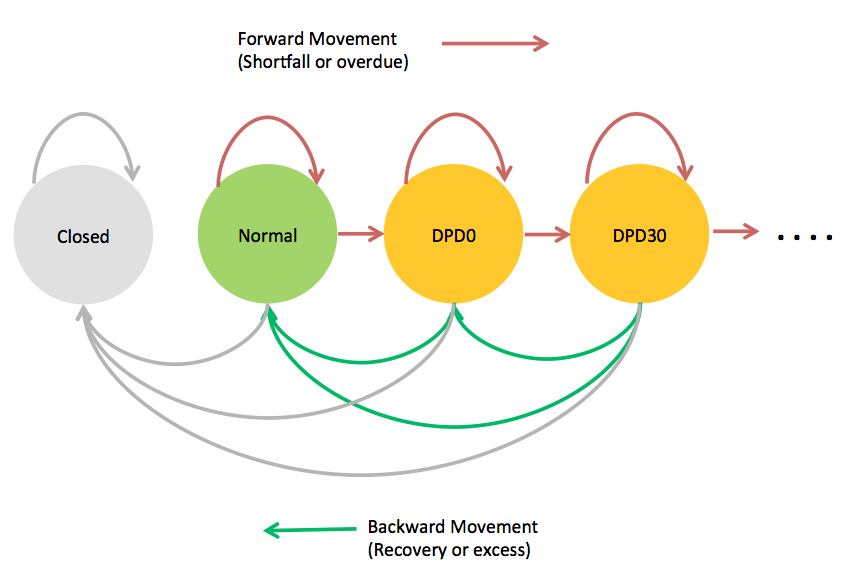
Figure 1: Possible transitions for a loan
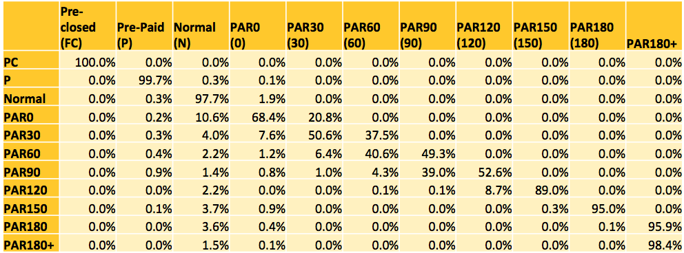
Figure 2: Illustrative TM capturing the transition of loans over one repayment period
The transition matrix can be used to simulate the possible states for all the loans in a portfolio. Each simulation represents a set of paths for all the loans, which denotes a single state of the universe of all the possible states through which the portfolio can evolve during its life. Periodic cash flows and resulting shortfalls (or excess) are estimated using these transitions for each simulation.
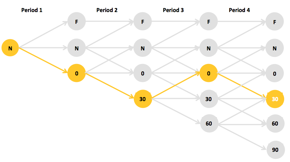
Figure 3: Simulating the path of a loan using TM
In this article which was published in the Securitisation & Structured Finance Handbook 2015/16, we present and discuss the TM-LGD model in some detail as well as its implementation and limitations through a case study based on the loss estimation for a securitization transaction with underlying commercial vehicle loans.
Click here to read the case study.